AIChE は American Institute of Chemical Engineers の略で、アメリカの化学工学会です。AIChE Annual Meeting はアメリカの化学工学会の年会なのですが、いろいろな国から参加者がいて、国際会議と化しています。43 ものディビジョン、フォーラムなどがあり、それぞれさらにいくつもセッションがあり、といった感じで非常に大きな会議です。
As industrial process plants, it is important to monitor product quality to assure both product quality and process safety. Soft sensors are models constructed between difficult-to-measure variables (y-variables) and easy-to-measure variables (X-variables). Values estimated with soft sensors are used to control plants rapidly. Partial least squares (PLS) [1] are the most popular linear regression methods. To handle nonlinear cases, support vector regression [2] and Gaussian process regression (GPR) [3] have been developed. Since the GPR method can generate a probabilistic model, an uncertainty estimation for the variable of interest can be obtained. However, the predictive ability of such techniques decreases due to process changes in chemical plants. To reduce the decrease of predictive ability, adaptive soft sensors have been developed [4]. We focus on just-in-time (JIT) soft sensors. The JIT model can be constructed online and can track process changes well. Locally weighted PLS (LWPLS) [5] is one of the nonlinear JIT methods. Since a set of hyperparameters in any JIT model has to be set beforehand and the hyperparameters of a JIT model will not always be the optimal ones for a query sample, the predictive ability of a JIT model decreases.
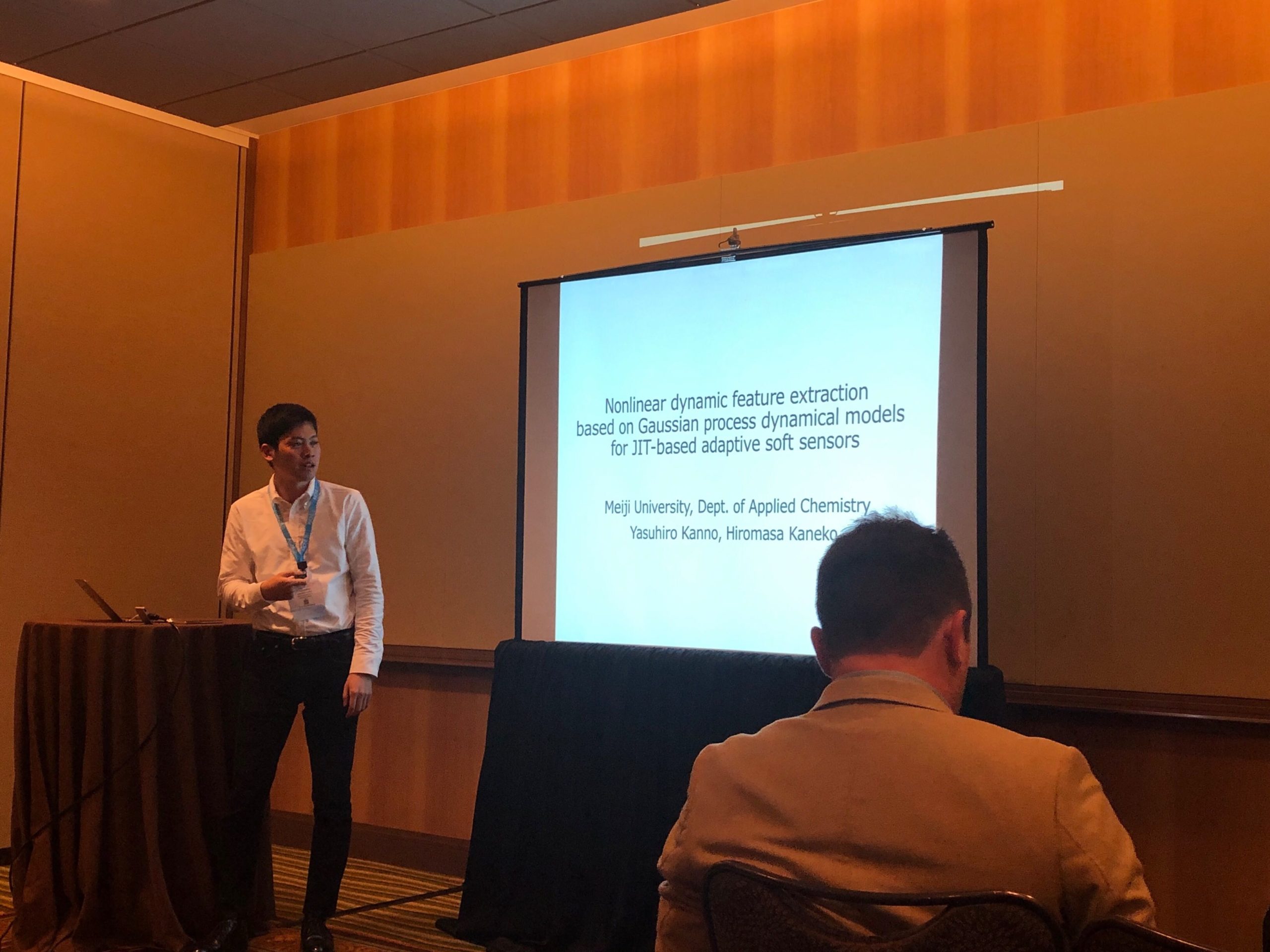
When constructing a soft sensor model for time series data, process dynamics are often considered to improve estimation performance [6]. In other words, not only the current time samples but also past samples are added to the X-variables to construct a model. On the other hand, if all these variables are used to construct the soft sensor model, it will increase the computation burden and make the model overfitting. Therefore, it is necessary to carry out dimensionality reduction and feature extraction before constructing the model. Principal component analysis (PCA) [7], as a traditional dimensionality reduction method, has been identified as an effective approach to transform observed variables to low-dimensional data. PCA is a linear method and developed in a deterministic manner, which lacks a probabilistic interpretation. As a matter of fact, process data are usually measured in a noisy environment and disturbances may happen. Also, there are nonlinearity between X-variables and temporal dependences between adjacent latent states and the data are autocorrelated. As an alternative, Gaussian process dynamical models (GPDM) [8] that is a nonlinear probabilistic dynamic latent variable model has been developed to model the process features. In GPDM, the latent states are assumed to be produced according to a first-order Markov chain, and each observation is generated from its current state by a nonlinear transformation. In this study, we propose to combine JIT and ensemble learning, and predict y-values with multiple JIT models, which are constructed using latent variables from GPDM and sets of hyperparameters are different. The proposed method is called ensemble just in time based on Gaussian process dynamical models (EJITGPDM). The weights of JIT models are determined based on Bayes’ theorem, considering their predictive ability. We check that the proposed model has higher predictive accuracy than traditional models through two industrial data analyses.
Proposed method
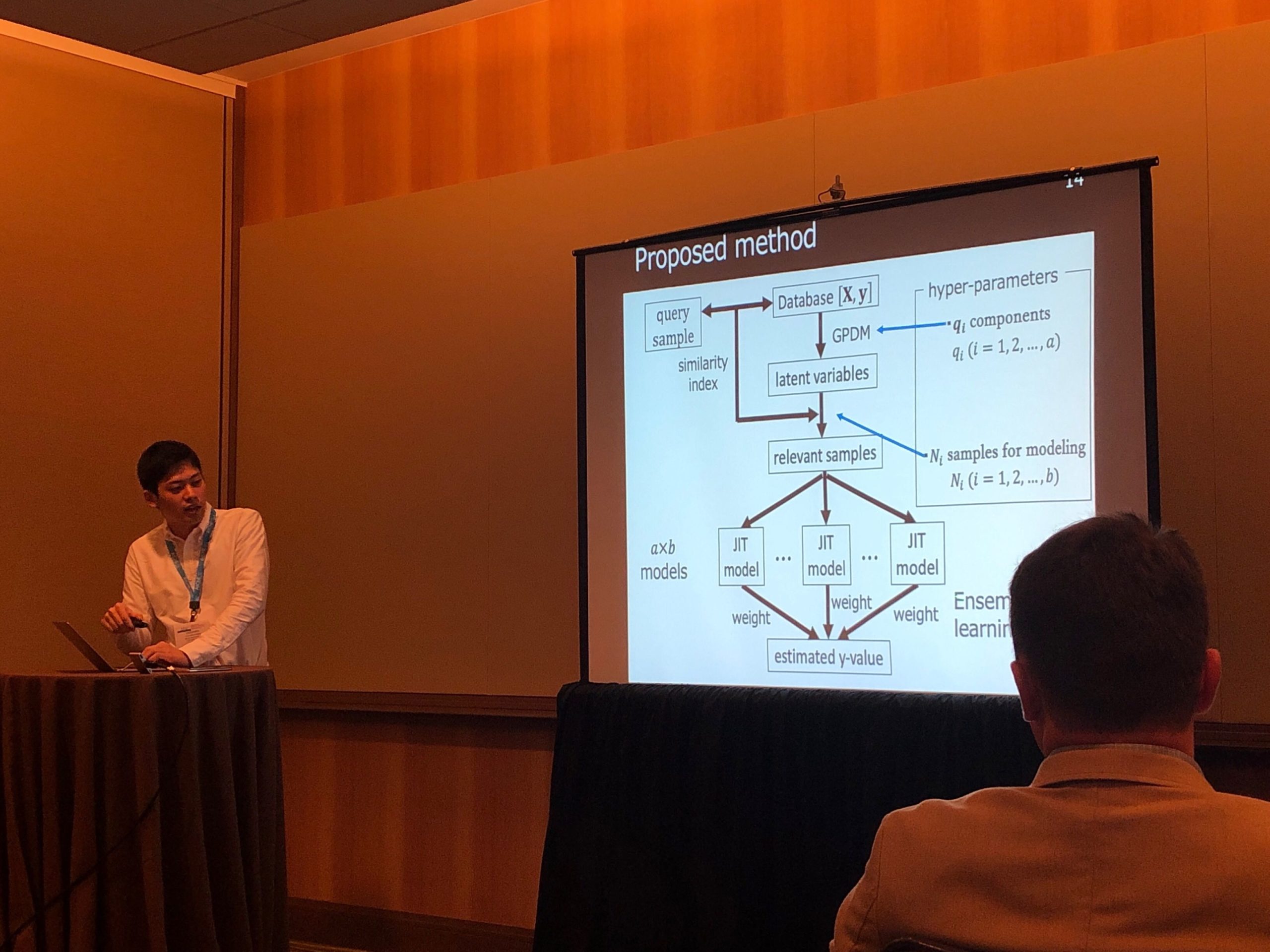
In the proposed method EJITGPDM, y-values are estimated from X-values by weighting the y-values predicted by multiple JIT models constructed using different hyperparameters. When a query sample xq comes, the Euclidean distance between each historical sample and the query sample is first calculated. Next, get the indexes of the N most relevant samples, which have a small Euclidean distance to the query sample. After extracting latent variables from GPDM, a GPR model is constructed between the latent variables of the sample with high similarity and y. In GPDM, it is necessary to determine the number of components, and in JIT model, the number of data for model construction. That is, when the number of GPDM components differs in m-values and the number of data for model construction differs in n-values, the number of JIT models is L (= m × n). The y-values for query sample are predicted with multiple JIT models, after that they are integrated with ensemble learning. Each weight of the predicted y-values are calculated with Bayesian theorem [9], taking into account the prediction ability of each JIT model. When S is the current (unobserved) state in a plant and Mi is the ith model, the probability of Mi given S, P(Mi|S), is required to combine the prediction results of L JIT models. Using RMSE for the mid-points between the k-nearest-neighbor data points for the s data, which is called RMSEmidknn [10], the predictive accuracy of nonlinear regression models can be evaluated. Therefore, using weight, that is, inverse of RMSEmidknn, y-values can be estimated while monitoring the predictive ability of each JIT model and weighting each model appropriately.
Results and Discussion
To verify the effectiveness of the proposed method, we analyzed two real industrial process datasets. The dynamic just in time based on Gaussian process regression model (DJIT-GPR) [11] and the dynamic LWPLS model (DLWPLS), the dynamic locally weighted principal component regression model (DLWPCR) [12] used for comparison.
Real industrial data in a debutanizer column [13]
We applied the proposed method to data obtained from the operation of a debutanizer column. The y-variable is the butane content in the bottom flow and the X-variables are top temperature, top pressure, reflux flow, flow to next process, sixth tray temperature and bottom temperature. We could use the dataset where the measurement intervals of the y-variable and the X-variables were 6 min and the measurement delay of the y-variables was 48 min. Data from 100 to 894 were used as training data and data from 895 to 1394 were used as validation data, and data from 1395 to 2394 were used as test data. Thus, we had 795 training data and 500 validation data, and 1394 test data.
The lowest r2 values was 0.401 whose DLWPCR model produced. Using the DJIT-GPR model and the DLWPLS model, prediction accuracy improved and their values were 0.840 and 0.856. Between DJIT-GPR, DLWPLS, DLWPCR, and EJITGPDM, the highest r2 was 0.898 whose EJITGPDM produced. The proposed model could predict y-values more accurately than the traditional models. The y-values predicted with the DLWPLS model have larger variation than those of the proposed EJITGPDM model, that is, the proposed EJITGPDM achieves stable and accurate prediction of y-values.
Real industrial data in a sulfur recovery unit (SRU) [14]
We applied the proposed method to data obtained from the operation of an SRU. The y-variable is the concentration of H2S in the tail gas of Line 4 and the X-variables are gas flow MEA GAS, air flow AIR MEA, secondary air flow AIR MEA 2, gas flow in SWS zone, air flow in SWS zone. In industrial process plants, there are a case where the measurement interval of y-variables is larger than the measurement interval of X-variables. We verified the effectiveness of the proposed method in the case where the measurement interval of y-variables is one sixth of the measurement interval of X-variables. Data from 100 to 4101 were used as training data and data from 4102 to 6099 were used as validation data, and data from 6070 to 3982 were used as test data. Thus, we had 667 training data and 333 validation data, and 3982 test data.
As was the case in the debutanizer column data, EJITGPDM produced the r2 value was the highest and its value was 0.693. It is more than 10% better than the value of DLWPLS. In time plots of actual y and estimated y for DLWPLS and EJITGPDM, The y-values, which were the unmeasured y-value part, have smaller variation than those of the comparison models.
Conclusions
We proposed the modeling method EJITGPDM, which takes into consideration the nonlinearity between X-variables and temporal dependences between adjacent latent states. Also, it is always possible to calculate predicted y-values of query samples using optimal hyperparameters. In order to verify the effectiveness of the proposed method, a case study was conducted using operation data measured by the debutanizer column, and operation data measured by the SRU. The simulation results show the effectiveness of the proposed method. Efficient and stable management and operation of chemical plants are expected by using the proposed method.
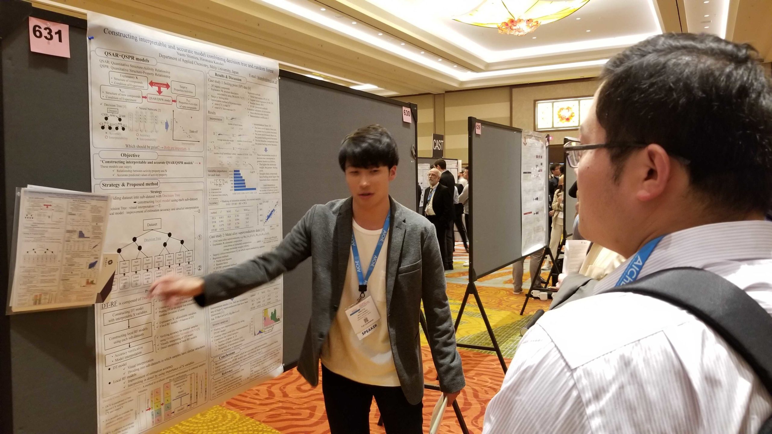
The estimation of properties and activities using machine learning has been actively performed. Quantitative structure-activity relationship (QSAR) and quantitative structure-property relationship (QSPR) models estimate activities and properties from chemical structures of compounds, respectively. Numerous methods for model construction have been developed for QSAR and QSPR models to have high accuracy and predictive ability. For example, partial least squares (PLS) [1], support vector regression (SVR) [2] and artificial neural networks (ANN) [3]. In 2004, organization for economic co-operation and development (OECD) determined 5 principles for the validation of QSAR models [4]: (i) a defined endpoint, (ii) an unambiguous algorithm, (iii) a defined domain of applicability, (iv) appropriate measures of goodness-of–fit, robustness and predictivity, (v) a mechanistic interpretation, if possible. Principles (i) ~ (iv) have been sufficiently investigated and it is possible to establish highly accurate model for samples in applicability domain, however, it is difficult to interpret highly accurate models. Model interpretation means discovering rules and mechanisms concerning specific physical properties and activities from models. There is room to research on interpretability of highly accurate models. Although examples of attempting to discover new mechanisms by interpreting models have been reported [5~8], there are three problems: interpretation is complicated, mechanisms cannot provide guidelines of syntheses and pursuing high interpretability leads to low accuracy. We aim to construct models with both highly predictive performance and high interpretability and solve the problem of the trade-off between accuracy and interpretability. We develop a new method combining an interpretable decision tree and regression methods.
Method
Decision tree (DT) [9] is a nonparametric regression analysis method that is based on a recursive partitioning of data using an explanatory variables X. In partitioning of data, data is divided into two subsets according to the value of X where objective variable y becomes as homogeneous as possible. A simple model structure like a tree enables visual interpretation. However, because of low computational complexity of decision tree, prediction accuracy is not very high.
Random forest (RF) [10] is an ensemble machine learning method that consists of many decision trees. y value is generated by summarizing all DT’s results. Each DT in RF model is independent and constructed with training samples randomly selected from all X variables. RF has an advantage that is to calculate feature importance which indicates the impact on estimation. Feature importance is measured how much the estimation accuracy decreases when permuting values of the feature.
The proposed method is composed of a DT and RF, which is named DT-RF. First, a dataset is divided into sub-datasets with DT, and local RF models are constructed using each sub-data sets. DT-RF model is possible to visually interpret a DT and local RF models increase estimation accuracy. In addition, local RF models can be interpreted in detail by using importance of X variables.
Result and discussion
Through case studies using superconductor data, we checked estimation accuracy, interpretability of model constructed with our proposed method and validity of the interpretation. Superconductor data extracted from the SuperCon [11] database is 15542 inorganic compounds data with critical temperature (Tc) at which superconductivity appears was measured. We used elemental composition, cross-terms of elemental composition and average molecular weight (AWM) as X variables to estimate Tc.
As a result of interpretation of constructed DT, we obtained following relationship between Tc and X variables:
(a) If not is equal to 0, a ratio of high Tc compounds is high.
(b) Tc of compounds whose composition ratio of oxygen is more than 0.5 is not so high.
(c) If is more than 0.011, a ratio of high Tc compounds is high.
In the previous research, La-Ba-Cu-O, Ba-Y-Cu-O, Bi-Sr-Ca-Cu-O, Tl-Ba-Ca-Cu-O and Hg-Ba-Cu-O alloy-based superconductor was discovered as high-temperature superconductors (Tc > 70[K]) [12, 13]. Interpretation result (a) and (c) are included in any of high-temperature superconductors that have been discovered. Estimation accuracy was evaluated by using coefficient of determination (r2) and mean absolute error (MAE). r2 and MAE in were 0.782 and 9.88, and r2 and MAE in CV were 0.732 and 11.0, respectively.
Local RF models were constructed with terminal subsets of DT model and predictive ability of local model was evaluated by double cross validation (DCV) [13], which is one of the methods to evaluate estimator performance in external dataset. DCV procedure is as follows:
(1) Dividing data at random, and one of the group is used for accuracy test, and the other groups are used for model construction.
(2) Optimization of hyperparameter in CV (inner-CV) and model construction using the groups for model construction.
(3) Estimation y value of a test group using the model built at (2).
(4) (1) ~ (3) is performed until all the groups used as test group (outer-CV).
(5) Comparing estimated y value calculated at (4) with measured y values to evaluate accuracy.
When constructing model in the case of a small number of samples and using CV for model optimization, hyperparameter are determined to improve the accuracy of y value in CV. The model fits into only samples for model construction and predictive ability for external data may not be adequately evaluated. On the other hand, DCV is composed of two nested CV referred to inner-CV and outer-CV, therefore, it is possible to evaluate the predictive ability more adequately than CV.Using samples of the terminal sub-dataset of DT for model construction, the number of samples is small and overfitting may occur. Then, DCV is effective in evaluating the predictive ability of the model adequately.
The estimation results of DCV using DT-RF and RF were MAE = 7.10, r2 = 0.866 and MAE = 7.51, r2 = 0.823, respectively. Thus, local RF models fit into sub-dataset in more detail than entire RF model. In particular, the samples with high Tc was estimated well. These results indicate that DT-RF is effectively used to discover new alloy materials with high Tc. According to local RF model of the highest Tc group in DT, Hg×O was chosen the most important X variable.
Conclusion
In this research, we developed a QSAR / QSPR model construction method with high interpretability and estimation accuracy. Instead of constructing a global model, local models were constructed using sub-datasets divided with DT, which made it possible to visually interpret the DT model and to predict y-values with high accuracy because local models fit into sub-datasets in more detail than an entire model. Since the small number of samples for model construction often heighten possibility of overfitting, we adopted DCV to adequately evaluate predictive ability of models. As a result of analyzing superconductor data with the proposed method, high prediction accuracy was achieved and interpretability and the validity was high because results of interpretation using DT corresponded to the superconductors that have been discovered. Interpreting local RF models, we obtain some important X variables that seem to deeply involve in the rise of Tc. We plan to new superconductors with high critical temperature by inverse analysis.
References
[1] P. Geladi; B. R. Kowalski, ANALYTICA CHIMICA ACTA, 1986
[2] R. Tibshirani, Journal of the Royal Statistical Society, 1996
[3] D.C. Park ; M.A. El-Sharkawi ; R.J. Marks ; L.E. Atlas ; M.J. Damborg, IEEE, 1991
[4] OECD Homepage Validation of (Q)SAR Models, http://www.oecd.org/chemicalsafety/risk-assessment/validationofqsarmodels.htm , 21 Oct 2018
[5] Supratik Kar; Juganta K. Roy; Danuta Leszczynska; Jerzy Leszczynski, MDPI, 2017
[6] Valentin Stanev; Corey Oses; A. Gilad Kusne; Efrain Rodriguez; Johnpierre Paglione; Stefano Curtarolo and Ichiro Takeuti; Machine learning modeling of superconducting critical temperature, ACS journal, 2018
[7] Vinicius M. Alves; Alexander Golbraikh; Stephan J. Capuzzi; Kammy Liu; Wai In Lam; Daniel Robert Korn; Diane Poze Approachfsky; Carolina Horta Andrade; Eugene N. Muratov and Alexander Tropsha, JCIM 2018, 58,1214-1223
[8] Ieda Maria dos Santos; Joao Pedro Gomes Agra; Thiego Gustavo Cavalcante de Carvalho; Gabriela de Azevedo Maia; Edilson Beserra de Alencar Filho, Springer, 2018, 29, 1287-1297
[11] Corey Oses, Cormac Toher, and Stefano Curtarolo, MRS, BULLETIN VOLUME 43, SEPTEMBER 2018[12] S. S. P. Parkin, V. Y. Lee, E. M. Engler, A. I. Nazzal, T. C. Huang, C. Gorman, R. Savoy, R. Beyers, Phys. Rev. Lett., 60, 2539, 1988[13] A. Schilling, M. Cantoni, J. D. Guo, H. R. Ott, Nature, 363, 56, 1993
[12] S. S. P. Parkin, V. Y. Lee, E. M. Engler, A. I. Nazzal, T. C. Huang, C. Gorman, R. Savoy, R. Beyers, Phys. Rev. Lett., 60, 2539, 1988
[13] A. Schilling, M. Cantoni, J. D. Guo, H. R. Ott, Nature, 363, 56, 1993
In chemical plants, process variables such as temperature, pressure and concentration are managed and controlled for the purpose of quality control of products, improvement of production efficiency and management of abnormalities in plants. Process variables can be divided into variables X that are easy to be measured in real time and frequently, and variables Y that are difficult to be measured. Therefore, soft sensors are widely used to estimate the value of Y online. The soft sensor is a numerical model constructed between X and Y with past measurement data. The value of Y can be estimated in real time by inputting the value of X measured in real time to the model. An error exists for Y. Cross validation (CV) method is one of methods to evaluate errors or the performance of soft sensors. However, the CV method has the following problems.
It takes a long time to evaluate models if there are many samples
If the number of samples is low, the number of samples used for model construction in the CV method will be lower and the model will become unstable
It can’t evaluate an already built model
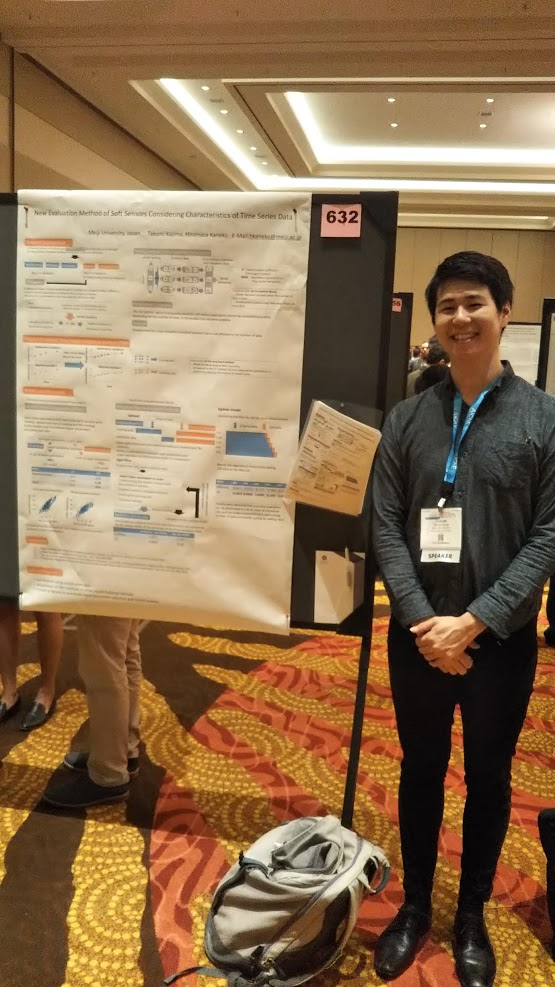
We aim to develop a new evaluation method that can solve these problems.
Proposed method
When selecting hyperparameters for model construction, a dataset is divided into training data and validation data. The model is constructed using only training data, and the accuracy of the model is confirmed using the verification data. However, depending on the number of original data, the constructed model tends to be unstable. In the proposed method, model construction is performed using all datasets. We propose middle points between training data and use them as temporary data for model validation. The proposed method enables model construction and evaluation using all data at one time. Since it is not necessary to repeat model construction as in the CV method, reduction of time required for evaluation is expected.
Results and Discussion
To verify the effectiveness of the proposed method, the simulation data of the plant Tennessee Eastman process (TEP) [1] and the two actual industrial process data sets Sulfur Recovery Unit (SRU) [2] and debutanizer column [3] were analyzed. The CV method and the proposed method were compared using support vector regression (SVR) [4] and recurrent neural network (RNN) [5] as regression analysis methods.
Tennessee Eastman Process (TEP) [3]
The effectiveness of the proposed method was verified using the simulation data of TEP. The regression method is SVR. The required hyperparameters for SVR were selected using CV method and the proposed method respectively, and the estimation performance and evaluation time of the constructed soft sensor were compared. The objective variable is the concentration of by-products. The explanatory variables used were 22 variables such as temperature and pressure.
10 samples in the dataset were used as training data for the purpose of evaluating the model created with a small number of data. In addition, there is randomness in the selection of training data, and the evaluation result of the model may be different at each analysis. Therefore, analysis was performed 10 times while changing data, and the average value of the obtained evaluation index was compared. The test data used 980 data from the data of TEP.
R2 was 0.430 for the CV method, and 0.508 for the proposed method. The time taken for the evaluation was 44.4 seconds in the CV method and 17.3 seconds in the proposed method. As a result, when the proposed method is used, the evaluation accuracy is improved, and the evaluation time is successfully shortened.
Sulfur Recovery Unit (SRU) [2]
The effectiveness of the proposed method was verified using the operation data obtained from the operation of SRU. The objective variable is the H2S concentration in the tail gas of line 4, The explanatory variables used were: gas flow MEA GAS, air flow AIR MEA, secondary air flow AIR MEA 2, gas flow in the SWS zone, and air flow in the SWS zone.
RNN, which is effective when the number of data is large, is used as the regression method. The selection of hyperparameters necessary for constructing RNN was performed using the proposed method. The number of times of learning was verified by using “early stopping” to determine whether learning can be stopped at an appropriate timing. The other hyperparameters were judged by comparing the evaluation accuracy of the soft sensor constructed by each of the cases with and without the proposed method.
The first two thirds of the data set were used as training data, and another one fifth was used when creating the validation data. In addition, the remaining one third of the initial data number was used as test data. Therefore, there were 6734 training data, 1374 validation data, and 3327 test data. Moreover, 6733 middle point data of all points in learning data were used as data for verification of the proposed method. As a result, we were able to select hyperparameters that could reduce the evaluation time while maintaining the model performance.
Debutanizer column [3]
The effectiveness of the proposed method was verified using the operating data obtained from the debutanizer operation. The target variable is the content of butane in the bottom stream. The explanatory variables used are: top temperature, top pressure, reflux flow, flow to next step, 6th tray temperature and bottom temperature.
The way to discuss the performance of the proposed method is the same as the way in SRU. There were 1266 training data, 317 validation data, and 791 test data. In addition, 1265 midpoint data of all points in the training data were used as data for verification of the proposed method. As a result, we were able to select hyperparameters that could reduce the evaluation time while maintaining the model performance.
Conclusions
The middle point between variables of time series data was constructed as validation data, and the evaluation method to evaluate the model was proposed. To verify the effectiveness of the proposed method, a case study was conducted using simulation data of TEP when the number of data is small, and operation data measured in SRU and data measured in debutanizer when there are many samples. As a result, regardless of the number of data, it was possible to select an appropriate hyperparameter and shorten the evaluation time. By using this proposed method, it is considered that stable and quick evaluation can be made possible by a soft sensor.
Reference
[1] LH Chiang, EL Russell, RD Braatz. Fault Detection and Diagnosis in Industrial Systems. Springer. 2001;103-112.
[4] Saneej B, Chitralekha, Sirish L Shah. Application of support vector regression for developing soft sensors for nonlinear processes. CSCHE. 2007;88:696-709.
[5] Seunghyun Han, Taekyoung Kim, Dooyoung Kim, Yong-Lae Park, Sungho Jo. Use of Deep Learning for Characterization of Microfluidic Soft Sensors. IEEE ROBO. 2018;3:873-880.