
こちらのDCEKit (Data Chemical Engineering toolKit) について、
クラスや関数の解説をします。少し長いですが、「Ctrl + F」で知りたいクラス・関数の名前を検索してもらえるとうれしいです。黄色のマーカーで強調されたクラス・関数について、それぞれ下に使い方の説明や使用例があります。scikit-learn の説明の仕方に似せたものにいます。
ちなみに、使用例である Examples の py ファイルは Github のページ

にあります!
class dcekit.generative_model.GTM(shape_of_map=[30, 30], shape_of_rbf_centers=[10, 10], variance_of_rbfs=4, lambda_in_em_algorithm=0.001, number_of_iterations=200, display_flag=1, sparse_flag=False)
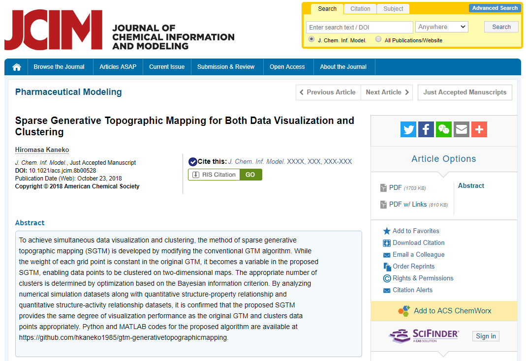
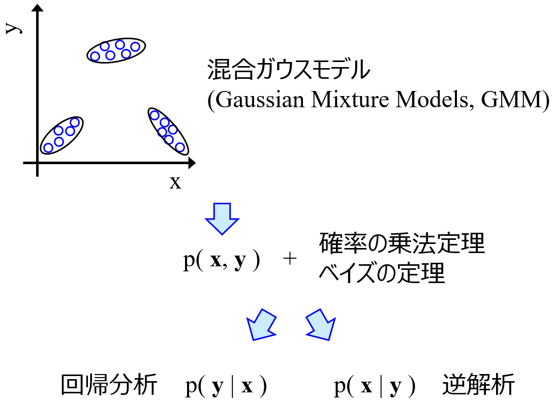
Generative Topographic Mapping (GTM)
Sparse Generative Topographic Mapping (SGTM)
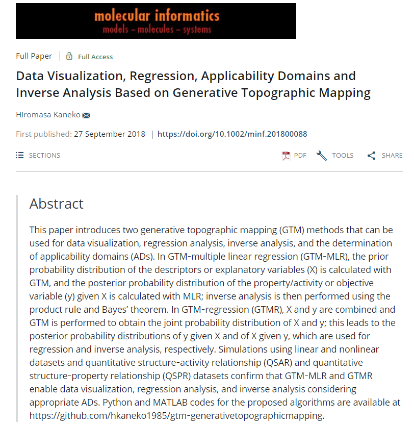
Generative Topographic Mapping Regression (GTMR)
Parameters:
- shape_of_map : list, optional, default [30, 30]
GTMマップのサイズ。[30, 30] のように list で [縦のサイズ, 横のサイズ] としてください - shape_of_rbf_centers : list, optional, default [10, 10]
RBF の数。[10, 10] のように list で [縦の数, 横の数] としてください - variance_of_rbfs : float, optional default 4
RBF の分散 - lambda_in_em_algorithm : float, optional, default 0.001
EM アルゴリズムにおけるラムダ - number_of_iterations : int, optional, default 200
EM アルゴリズムにおける繰り返し回数 - display_flag : boolean, optional, default True
True のとき EM アルゴリズムにおける途中結果が表示されます。途中結果を表示させたくないときは False としてください - sparse_flag=False : boolearn, optional, default False
False のとき GTM (もしくはGTMR) になります。GTM ではなく SGTM (もしくは SGTM Regression) を実行したいときは True としてください
Attributes:
- map_grids : array, shape shape_of_map
GTM マップのグリッド点の座標 - rbf_grids : array, shape shape_of_rbf_centers
RBF の座標 - W
GTM における W - beta
GTM における β
Methods:
- fit(self, input_dataset) : Fit GTM, SGTM and GTMR model
- fit_transform(self, x, mean_flag=True) : Fit GTM and SGTM, and transform x
- transform(self, x, mean_flag=True) : Transform x using constructed GTM and SGTM model
- responsibility(self, input_dataset) : Calculate responsibility
- means_modes(self, input_dataset): Calculate means and modes
- likelihood(self, input_dataset) : Calculate likelihood
- predict(self, input_variables, numbers_of_input_variables, numbers_of_output_variables) : Predict values of variables for forward analysis (regression) and inverse analysis using the GTMR model
- cv_opt(self, dataset, numbers_of_input_variables, numbers_of_output_variables, candidates_of_shape_of_map, candidates_of_shape_of_rbf_centers, candidates_of_variance_of_rbfs, candidates_of_lambda_in_em_algorithm, fold_number, number_of_iterations) : Optimize hyperparameter values of GTMR model using cross-validation
fit(self, input_dataset)
Fit GTM, SGTM and GTMR model
Parameters :
- input_dataset : numpy.array or pandas.DataFrame, shape (n_samples, n_features)
GTM モデル構築のための (オートスケーリング後の) トレーニングデータ。GTMRでは x, y を横に繋げて input_dataset としてください
Returns :
- self : returns an instance of self
scikit-learn と同じ感じです
fit_transform(self, x)
Fit GTM and SGTM, and transform x
Parameters :
- x: numpy.array or pandas.DataFrame, shape (n_samples, n_features)
GTM モデルを構築して写像させるための (オートスケーリング後の) トレーニングデータ - mean_flag: boolean, default True
True のとき mean, False のとき mode を返します
Returns :
- means or modes: numpy.array, shape (n_samples, 2)
means もしくは modes の座標
transform(self, x)
Transform x using constructed GTM and SGTM model
Parameters :
- x: numpy.array or pandas.DataFrame, shape (n_samples, n_features)
写像するための (オートスケーリング後の) データ - mean_flag: boolean, default True
True のとき mean, False のとき mode を返します
Returns :
- means or modes: numpy.array, shape (n_samples, 2)
means もしくは modes の座標
responsibility(self, input_dataset)
Calculate responsibility
Parameters :
- input_dataset : numpy.array or pandas.DataFrame, shape (n_samples, n_features)
Responsibility を計算する (オートスケーリング後の) データ。fit したデータと変数の数 (n_features) を同じにしてください
Returns :
- reponsibilities : numpy.array
グリッド点ごとの responsibility の値
means_modes(self, input_dataset)
Calculate means and modes
Parameters :
- input_dataset : numpy.array or pandas.DataFrame, shape (n_samples, n_features)
means と modes を計算する (オートスケーリング後の) データ。fit したデータと変数の数 (n_features) を同じにしてください
Returns :
- means : numpy.array, shape (n_samples, 2)
means の座標 - modes : numpy.array, shape (n_samples, 2)
modes の座標
likelihood(self, input_dataset)
Calculate likelihood
Parameters :
- input_dataset : numpy.array or pandas.DataFrame, shape (n_samples, n_features)
likelihood を計算する (オートスケーリング後の) データ。fit したデータと変数の数 (n_features) を同じにしてください
Returns :
- likelihood : float
likelihood
predict(self, input_variables, numbers_of_input_variables, numbers_of_output_variables)
Predict values of variables for forward analysis (regression) and inverse analysis using the GTMR model
Parameters :
- input_variables: numpy.array or pandas.DataFrame, shape (n_samples, n_features or n_targets)
予測用の (オートスケーリング後の) データ。次の input_variables で指定する変数番号の数 (ベクトルの大きさ) と変数の数 (n_features) を同じにしてください。説明変数 X のデータのとき順解析、目的変数Yのデータのとき逆解析になります。 - numbers_of_input_variables: list or numpy.array, shape (n_features or n_targets,)
fit したデータの変数に対応する上の input_variables の変数番号を、list か array のベクトルで与えてください。たとえば fit したデータが 5 変数あり、input_variables として入力するデータが 3 変数で 0, 1, 2 番目の変数のとき、numbers_of_input_variables = [0, 1, 2] となります。これが X の変数番号であれば順解析、Y の変数番号であれば逆解析になります - numbers_of_output_variables : list or numpy.array, shape (n_targets or n_features,)
fit したデータの変数に対応する予測したい変数番号を、list か array のベクトルで与えてください。たとえば fit したデータが 5 変数あり、予測したい変数が 2 変数で 3, 4 番目の変数のとき、numbers_of_output_variables = [3, 4] となります。これが Y の変数番号であれば順解析、X の変数番号であれば逆解析になります
Returns :
- mode_of_estimated_mean : numpy.array, shape (n_samples, n_targets or n_features)
weights の modes で与えられる numbers_of_output_variables の推定値 - weighted_estimated_mean : numpy.array, shape (n_samples, n_targets or n_features)
weights の means (重み付き平均) で与えられる numbers_of_output_variables の推定値 - estimated_mean_for_all_components : numpy.array, shape (n_grids, n_samples, n_targets or n_features)
Grid 点ごとの numbers_of_output_variables の推定値 - weights : numpy.array, shape (n_samples, n_grids)
Grid 点ごとの重み
Examples :
- GTM :
- demo_gtm.py
- demo_opt_gtm_with_k3nerror.py (k3n error を用いた GTM のハイパーパラメータの最適化)
- SGTM :
- demo_sgtm.py
- GTMR :
- demo_gtmr.py
- demo_gtmr_multi_y.py (目的変数が複数)
- demo_opt_gtmr_with_cv_multi_y.py (クロスバリデーションによるハイパーパラメータの最適化、目的変数が複数)
- demo_opt_gtmr_with_cv_multi_y_descriptors.py (クロスバリデーションによるハイパーパラメータの最適化、目的変数が複数、化合物のデータ)
- demo_inverse_gtmr.py (モデルの逆解析)
- demo_inverse_gtmr_with_multi_y.py (モデルの逆解析、目的変数が複数)
class dcekit.generative_model.GMR(covariance_type=’full’, n_components=10, rep=’mean’ max_iter=100, random_state=None, display_flag=False)
sklearn.mixture.GaussianMixture を継承しています。
Gaussian Mixture Regression (GMR)

Parameters:
- n_components : int, default 10
正規分布の数 - covariance_type : {‘full’ (default), ‘tied’, ‘diag’, ‘spherical’}
分散共分散行列の種類。’full’ : すべての正規分布の分散・共分散は自由。’tied’ : すべての正規分布において分散・共分散が同じ。’diag’ : すべての正規分布の共分散が 0、分散は自由。’spherical’ : すべての正規分布の分散が 1、共分散が 0 - rep : (predict_repで予測する用) {‘mean’ (default), ‘mode’}
予測値の代表値の計算方法。’mean’ : 各正規分布の平均値の重み付き平均。’mode’ : 重みが最大の正規分布の平均値 - max_iter : int, default 100
EM アルゴリズムの繰り返し回数 - random_state : int, RandomState instance or None, optional (default=None)
この整数を同じにすると結果に再現性があります - display_flag : boolean, optional, default True
True のときクロスバリデーションにおける途中結果が表示されます。途中結果を表示させたくないときは False としてください
Attributes:
- weights_ : numpy.array, shape (n_components,)
各正規分布の重み - means_ : numpy.array, shape (n_components, n_features)
各正規分布の平均
Methods:
- fit(self, input_dataset) : Fit GMR model
- predict(self, input_variables, numbers_of_input_variables, numbers_of_output_variables) : Predict values of variables for forward analysis (regression) and inverse analysis using the GMR model
- predict_rep(self, input_variables, numbers_of_input_variables, numbers_of_output_variables) : Predict values of variables for forward analysis (regression) and inverse analysis using the GMR model. The way to calculate representative values can be set with ‘rep’
- cv_opt(self, dataset, numbers_of_input_variables, numbers_of_output_variables, covariance_types, numbers_of_components, fold_number) : Optimize hyperparameter values of GMR model using cross-validation
fit(self, input_dataset)
Fit GMR model
Parameters :
- input_dataset : numpy.array or pandas.DataFrame, shape (n_samples, n_features)
GMR モデル構築のための (オートスケーリング後の) トレーニングデータ。GMRでは x, y を横に繋げて input_dataset としてください
Returns :
- self : returns an instance of self
scikit-learn と同じです
predict(self, input_variables, numbers_of_input_variables, numbers_of_output_variables)
Predict values of variables for forward analysis (regression) and inverse analysis using the GMR model
Parameters :
- input_variables: numpy.array or pandas.DataFrame, shape (n_samples, n_features or n_targets)
予測用の (オートスケーリング後の) データ。次の input_variables で指定する変数番号の数 (ベクトルの大きさ) と変数の数 (n_features) を同じにしてください。説明変数 X のデータのとき順解析、目的変数Yのデータのとき逆解析になります。 - numbers_of_input_variables: list or numpy.array, shape (n_features or n_targets,)
fit したデータの変数に対応する上の input_variables の変数番号を、list か array のベクトルで与えてください。たとえば fit したデータが 5 変数あり、input_variables として入力するデータが 3 変数で 0, 1, 2 番目の変数のとき、numbers_of_input_variables = [0, 1, 2] となります。これが X の変数番号であれば順解析、Y の変数番号であれば逆解析になります - numbers_of_output_variables : list or numpy.array, shape (n_targets or n_features,)
fit したデータの変数に対応する予測したい変数番号を、list か array のベクトルで与えてください。たとえば fit したデータが 5 変数あり、予測したい変数が 2 変数で 3, 4 番目の変数のとき、numbers_of_output_variables = [3, 4] となります。これが Y の変数番号であれば順解析、X の変数番号であれば逆解析になります
Returns :
- mode_of_estimated_mean : numpy.array, shape (n_samples, n_targets or n_features)
weights の modes で与えられる numbers_of_output_variables の推定値 - weighted_estimated_mean : numpy.array, shape (n_samples, n_targets or n_features)
weights の means (重み付き平均) で与えられる numbers_of_output_variables の推定値 - estimated_mean_for_all_components : numpy.array, shape (n_grids, n_samples, n_targets or n_features)
正規分布ごとの numbers_of_output_variables の推定値 - weights : numpy.array, shape (n_samples, n_grids)
正規分布ごとの重み
Examples :
- demo_gmr.py (回帰分析、モデルの逆解析、目的変数が複数)
- demo_gmr_with_cross_validation.py (クロスバリデーションによるハイパーパラメータの最適化)
- demo_gmr_with_interpolation.py (欠損値の補完)
class dcekit.generative_model.VBGMR(covariance_type=’full’, n_components=30, weight_concentration_prior_type=’dirichlet_process’, weight_concentration_prior=0.01, rep=’mean’, max_iter=100, random_state=None, display_flag=False)
sklearn.mixture.BayesianGaussianMixture を継承しています。
Variational Bayesian Gaussian Mixture Regression (VBGMR)
Parameters:
- n_components : int, default 30
正規分布の数 - covariance_type : {‘full’ (default), ‘tied’, ‘diag’, ‘spherical’}
分散共分散行列の種類。’full’ : すべての正規分布の分散・共分散は自由。’tied’ : すべての正規分布において分散・共分散が同じ。’diag’ : すべての正規分布の共分散が 0、分散は自由。’spherical’ : すべての正規分布の分散が 1、共分散が 0 - weight_concentration_prior_type : {‘dirichlet_process’ (default), ‘dirichlet_distribution’}
正規分布の重みの事前分布。’dirichlet_process’ : ディリクレ過程。’dirichlet_distribution’ : ディリクレ分布 - weight_concentration_prior : float, default 0.01
正規分布の重みの事前分布のパラメータ - rep : (predict_repで予測する用) {‘mean’ (default), ‘mode’}
予測値の代表値の計算方法。’mean’ : 各正規分布の平均値の重み付き平均。’mode’ : 重みが最大の正規分布の平均値 - max_iter : int, default 100
EM アルゴリズムの繰り返し回数 - random_state : int, RandomState instance or None, optional (default=None)
この整数を同じにすると結果に再現性があります - display_flag : boolean, optional, default True
True のときクロスバリデーションにおける途中結果が表示されます。途中結果を表示させたくないときは False としてください
Attributes:
- weights_ : numpy.array, shape (n_components,)
各正規分布の重み - means_ : numpy.array, shape (n_components, n_features)
各正規分布の平均
Methods:
- fit(self, input_dataset) : Fit VBGMR model
- predict(self, input_variables, numbers_of_input_variables, numbers_of_output_variables) : Predict values of variables for forward analysis (regression) and inverse analysis using the VBGMR model
- predict_rep(self, input_variables, numbers_of_input_variables, numbers_of_output_variables) : Predict values of variables for forward analysis (regression) and inverse analysis using the VBGMR model. The way to calculate representative values can be set with ‘rep’
- cv_opt(self, dataset, numbers_of_input_variables, numbers_of_output_variables, covariance_types, numbers_of_components, weight_concentration_prior_types, weight_concentration_priors, fold_number) : Optimize hyperparameter values of VBGMR model using cross-validation
fit(self, input_dataset)
Fit VBGMR model
Parameters :
- input_dataset : numpy.array or pandas.DataFrame, shape (n_samples, n_features)
VBGMR モデル構築のための (オートスケーリング後の) トレーニングデータ。GMRでは x, y を横に繋げて input_dataset としてください
Returns :
- self : returns an instance of self
scikit-learn と同じです
predict(self, input_variables, numbers_of_input_variables, numbers_of_output_variables)
Predict values of variables for forward analysis (regression) and inverse analysis using the VBGMR model
Parameters :
- input_variables: numpy.array or pandas.DataFrame, shape (n_samples, n_features or n_targets)
予測用の (オートスケーリング後の) データ。次の input_variables で指定する変数番号の数 (ベクトルの大きさ) と変数の数 (n_features) を同じにしてください。説明変数 X のデータのとき順解析、目的変数Yのデータのとき逆解析になります。 - numbers_of_input_variables: list or numpy.array, shape (n_features or n_targets,)
fit したデータの変数に対応する上の input_variables の変数番号を、list か array のベクトルで与えてください。たとえば fit したデータが 5 変数あり、input_variables として入力するデータが 3 変数で 0, 1, 2 番目の変数のとき、numbers_of_input_variables = [0, 1, 2] となります。これが X の変数番号であれば順解析、Y の変数番号であれば逆解析になります - numbers_of_output_variables : list or numpy.array, shape (n_targets or n_features,)
fit したデータの変数に対応する予測したい変数番号を、list か array のベクトルで与えてください。たとえば fit したデータが 5 変数あり、予測したい変数が 2 変数で 3, 4 番目の変数のとき、numbers_of_output_variables = [3, 4] となります。これが Y の変数番号であれば順解析、X の変数番号であれば逆解析になります
Returns :
- mode_of_estimated_mean : numpy.array, shape (n_samples, n_targets or n_features)
weights の modes で与えられる numbers_of_output_variables の推定値 - weighted_estimated_mean : numpy.array, shape (n_samples, n_targets or n_features)
weights の means (重み付き平均) で与えられる numbers_of_output_variables の推定値 - estimated_mean_for_all_components : numpy.array, shape (n_grids, n_samples, n_targets or n_features)
正規分布ごとの numbers_of_output_variables の推定値 - weights : numpy.array, shape (n_samples, n_grids)
正規分布ごとの重み
Examples :
- demo_vbgmr.py (回帰分析、モデルの逆解析、目的変数が複数)
- demo_vbgmr_with_cross_validation.py (クロスバリデーションによるハイパーパラメータの最適化)
dcekit.validation.k3nerror(x1, x2, k)
k3n error (k–nearest neighbor normalized error for visualization and reconstruction)
When x1 is data of X-variables and x2 is data of Z-variables (low-dimensional data), this is k3n error in visualization (k3n-Z-error). When x1 is Z-variables (low-dimensional data) and x2 is data of data of X-variables, this is k3n error in reconstruction (k3n-X-error).
k3n-error = k3n-Z-error + k3n-X-error
Parameters :
- x1 : numpy.array or pandas.DataFrame, shape (n_samples, n_features or n_latent_variables)
オリジナルの変数の (オートスケーリング後の) データセット、もしくは低次元化後 (可視化後) のデータセット - x2 : numpy.array or pandas.DataFrame, shape (n_samples, n_latent_variables or n_features)
低次元化後 (可視化後) のデータセット、もしくはオリジナルの変数の (オートスケーリング後の) データセット - k : int, default 10
用いる最近傍点の数
Returns :
- k3nerror : float
k3n-Z-error もしくは k3n-X-error
Examples :
- demo_opt_gtm_with_k3nerror.py
dcekit.validation.midknn(x, k)
midpoints between k-nearest-neighbor data points of a training dataset (midknn)
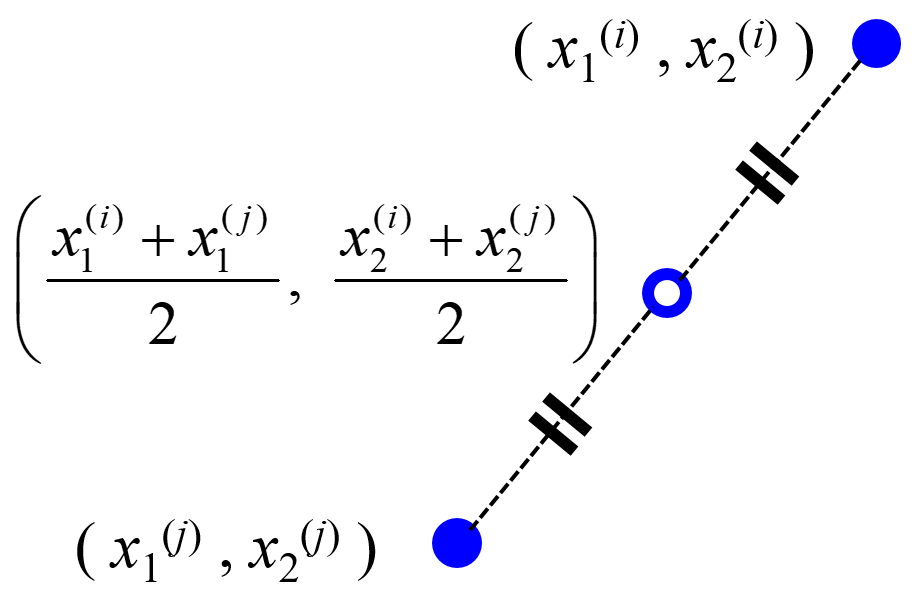
Calculate index of midknn of training dataset for validation dataset in regression
Parameters :
- x : numpy.array or pandas.DataFrame, shape (n_samples, n_features)
(オートスケーリング後の) データセット - k : int, default 10
用いる最近傍点の数
Returns :
- midknn : numpy.array
midknn を計算する 2 つのサンプルの番号
dcekit.validation.make_midknn_dataset(x, y, k)
Get dataset of midknn
Parameters :
- x : numpy.array or pandas.DataFrame, shape (n_samples, n_features)
(オートスケーリング後の) X のデータセット - y : numpy.array or pandas.DataFrame, shape (n_samples,)
(オートスケーリング後の) Y のデータセット - k : int, default 10
用いる最近傍点の数
Returns :
- x_midknn : numpy.array
X の midknn - y_midknn : numpy.array
Y の midknn
Examples :
- demo_midknn_in_svr.py
- demo_fast_opt_svr_hyperparams_midknn.py
dcekit.validation.double_cross_validation(gs_cv, x, y, outer_fold_number, do_autoscaling=True, random_state=None)
ダブルクロスバリデーション (Double Cross-Validation, DCV)

Estimate y-values in DCV
Parameters :
- gs_cv : object of GridSearchCV (sklearn.model_selection.GridSearchCV)
sklearn でクロスバリデーションするときの GridSearchCV を設定して入力してください。内側のクロスバリデーションで使用します - x : numpy.array or pandas.DataFrame, shape (n_samples, n_features)
(オートスケーリング前の) X のデータセット - y : numpy.array or pandas.DataFrame, shape (n_samples,)
(オートスケーリング前の) Y のデータセット - outer_fold_number : int
外側のクロスバリデーションにおける fold 数。x, y のサンプル数にすると、外側は leave-one-out クロスバリデーションになります - do_autoscaling : boolean, optional, default True
True のとき外側のクロスバリデーションでオートスケーリングします。オートスケーリングしたくないときは False にしてください - random_state : int, RandomState instance or None, optional (default=None)
この整数を同じにすると結果に再現性があります
Returns :
- estimated_y : numpy.array
DCV における Y の推定値
Examples :
- demo_double_cross_validation_for_pls.py (PLS)
dcekit.validation.y_randomization(model, x, y, do_autoscaling=True, random_state=None)
y-randomization or y-scrambling

Estimated y-values after shuffling y-values of dataset without hyperparameters
Parameters :
- model : object of model in scikit-learn
sklearn で fit する前のモデルを準備して入力してください - x : numpy.array or pandas.DataFrame, shape (n_samples, n_features)
(オートスケーリング前の) X のデータセット - y : numpy.array or pandas.DataFrame, shape (n_samples,)
(オートスケーリング前の) Y のデータセット - do_autoscaling : boolean, optional, default True
True のときオートスケーリングします。オートスケーリングしたくないときは False にしてください - random_state : int, RandomState instance or None, optional (default=None)
この整数を同じにすると結果に再現性があります
Returns :
- y_shuffle : numpy.array, shape (n_samples,)
シャッフルされた Y のデータセット - estimated_y_shuffle : numpy.array
シャッフルされた Y の推定値
Examples :
- demo_y_randomization.py (OLS, GP)
dcekit.validation.y_randomization_with_hyperparam_opt(gs_cv, x, y, do_autoscaling=True, random_state=None):
y-randomization or y-scrambling
Estimated y-values after shuffling y-values of dataset with hyperparameters
Parameters :
- gs_cv : object of GridSearchCV (sklearn.model_selection.GridSearchCV)
sklearn でクロスバリデーションするときの GridSearchCV を設定して入力してください。Y をシャッフルした後のクロスバリデーションで使用します - x : numpy.array or pandas.DataFrame, shape (n_samples, n_features)
(オートスケーリング前の) X のデータセット - y : numpy.array or pandas.DataFrame, shape (n_samples,)
(オートスケーリング前の) Y のデータセット - do_autoscaling : boolean, optional, default True
True のときオートスケーリングします。オートスケーリングしたくないときは False にしてください - random_state : int, RandomState instance or None, optional (default=None)
この整数を同じにすると結果に再現性があります
Returns :
- y_shuffle : numpy.array, shape (n_samples,)
シャッフルされた Y の実測値 - estimated_y_shuffle : numpy.array
シャッフルされた Y の推定値
Examples :
- demo_y_randomization_with_hyperparameter.py (PLS)
dcekit.validation.mae_cce(gs_cv, x, y, number_of_y_randomization=30, do_autoscaling=True, random_state=None)
Chance Correlation‐Excluded Mean Absolute Error (MAECCE)
Calculate MAECCE
Parameters :
- gs_cv : object of GridSearchCV (sklearn.model_selection.GridSearchCV)
sklearn でクロスバリデーションするときの GridSearchCV を設定して入力してください。Y をシャッフルした後のクロスバリデーションで使用します - x : numpy.array or pandas.DataFrame, shape (n_samples, n_features)
(オートスケーリング前の) X のデータセット - y : numpy.array or pandas.DataFrame, shape (n_samples,)
(オートスケーリング前の) Y のデータセット - number_of_y_randomization : int, default 30
y-randomization をする回数 - do_autoscaling : boolean, optional, default True
True のときオートスケーリングします。オートスケーリングしたくないときは False にしてください - random_state : int, RandomState instance or None, optional (default=None)
この整数を同じにすると結果に再現性があります
Returns :
- mae_cce : numpy.array, shape (number_of_y_randomization,)
MAECCE の値のベクトル
Examples :
- demo_maecce_for_pls.py (PLS)
dcekit.validation.r2lm(measured_y, estimated_y)
r2 based on the latest measured y-values (r2LM)
Calculate r2LM
Parameters :
- measured_y: numpy.array or pandas.DataFrame, shape (n_samples,)
Y の実測値 - estimated_y: numpy.array or pandas.DataFrame, shape (n_samples,)
Y の推定値
Returns :
- r2lm : float
r2LM
Examples :
- demo_lwpls_r2lm.py
- demo_time_series_data_analysis_lwpls_r2lm.py
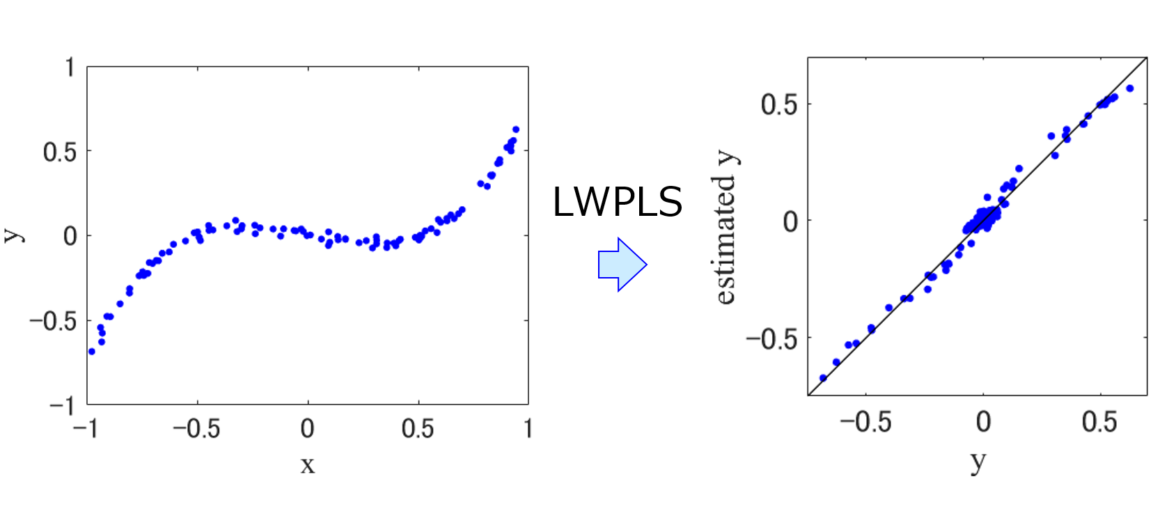
class dcekit.just_in_tme.LWPLS(n_components=2, lambda_in_similarity=1.0)
scikit-learn に準拠しています (GridSearchCV や cross_val_predict を使えます)。
Locally-Weighted Partial Least Squares (LWPLS, 局所PLS)
Parameters :
- n_components : int
LWPLS で使用する成分数 - lambda_in_similarity: float
類似度行列における λ
Methods:
- fit(self, X, y) : Store X and y as training data
- predict(self, X) : Train LWPLS model and predict values of X
fit(self, X, y) : Store X and y as training data
Parameters :
- X : numpy.array, shape (n_samples, n_features)
LWPLS モデル構築のための x のデータ - y : numpy.array, shape (n_samples,)
LWPLS モデル構築のための y のデータ
Returns :
- self : returns an instance of self
scikit-learn と同じです
predict(self, X) : Train LWPLS model and predict values of X
Parameters :
- X : numpy.array, shape (n_samples, n_features)
LWPLS モデルで予測するための x のデータ
Returns :
- estimated_y : numpy.array, shape (n_samples,)
y の予測値
Examples :
- demo_lwpls_r2lm.py
- demo_time_series_data_analysis_lwpls_r2lm.py (時系列データでの LWPLS)
dcekit.optimization.iot(x_mix, x_pure)
Iterative Optimization Technology (IOT)
Parameters :
- x_mix : numpy.array or pandas.DataFrame, shape (n_spectra, n_features)
混合物のスペクトル - x_pure : numpy.array or pandas.DataFrame, shape (n_materials, n_features)
純成分のスペクトル
Returns :
- pred_mol_fracs : numpy.array
混合物における各純成分の予測されたモル分率
Examples :
- demo_iot.py
dcekit.optimization.fast_opt_svr_hyperparams(x, y, cs, epsilons, gammas, validation_method, parameter)
サポートベクター回帰 (Support Vector Regression, SVR) のハイパーパラメータの高速最適化
Optimize SVR hyperparameters based on variance of gram matrix and cross-validation or midknn
Parameters :
- x : numpy.array or pandas.DataFrame, shape (n_samples, n_features)
(オートスケーリング後の) X のトレーニングデータ - y : numpy.array or pandas.DataFrame, shape (n_samples,)
(オートスケーリング後の) Y のトレーニングデータ - cs : numpy.array or list, shape (n_c,)
SVR における C の候補のベクトル - epsilons : numpy.array or list, shape (n_epsilon,)
SVR における ε の候補のベクトル - gammas : numpy.array or list, shape (n_gamma,)
SVR における γ の候補のベクトル - validation_method : ‘cv’ or ‘midknn’
‘cv’ のときクロスバリデーション使用、’midknn’ のとき midknn 使用 - parameter : int
クロスバリデーションのときクロスバリデーションの分割数、midknn のとき midknn における k の値
Returns :
- optimal_c : float
最適化された C の値 - optimal_epsilon : float
最適化された ε の値 - optimal_gamma : float
最適化された γ の値
Examples :
- demo_fast_opt_svr_hyperparams_cv.py (クロスバリデーション使用)
- demo_fast_opt_svr_hyperparams_midknn.py (midknn 使用)
dcekit.sampling.kennard_stone(dataset, number_of_samples_to_be_selected)
Kennard-Stone (KS) アルゴリズムによるサンプル選択
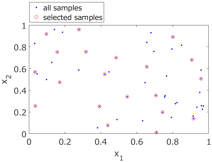
Select samples using KS algorithm
Parameters :
- dataset : numpy.array or pandas.DataFrame, shape (n_samples, n_features)
(オートスケーリング後の) データセット - number_of_samples_to_be_selected : int
選択するサンプルの数
Returns :
- selected_sample_numbers : list
選択されたサンプルのインデックス番号 (トレーニングデータのインデックス番号) - remaining_sample_numbers : list
選択されなかったサンプルのインデックス番号 (テストデータのインデックス番号)
Examples :
- demo_kennard_stone.py
dcekit.variable_selection.search_high_rate_of_same_values(x, threshold_of_rate_of_same_values)
同じ値をもつサンプルの割合が高い変数の探索

Search variables with high rate of the same values
Parameters :
- x : numpy.array or pandas.DataFrame, shape (n_samples, n_features)
(オートスケーリング前の) データセット - threshold_of_rate_of_same_values : float (0 ~ 1)
同じ値をもつサンプルの割合のしきい値。この値以上の割合をもつ変数を選択します
Returns :
- high_rate_variable_numbers : list
選択された (同じ値をもつサンプルの割合が高い) 変数の番号
Examples :
- demo_search_highly_correlated_variables.py
- demo_clustering_based_on_correlation_coefficients.py
dcekit.variable_selection.search_highly_correlated_variables(x, threshold_of_r)
相関係数 r に基づく変数選択
Search variables whose absolute correlation coefficient is higher than threshold_of_r
Parameters :
- x : numpy.array or pandas.DataFrame, shape (n_samples, n_features)
(オートスケーリング前の) データセット - threshold_of_r : float (0 ~ 1)
相関係数の絶対値のしきい値。変数間に、この値以上の相関係数の絶対値をもつ変数の組がなくなるまで変数を選択します
Returns :
- highly_correlated_variable_numbers : list
選択された (相関係数の絶対値の高い) 変数の番号
Examples :
- demo_search_highly_correlated_variables.py
dcekit.variable_selection.clustering_based_on_correlation_coefficients(x, threshold_of_r)
相関係数 r の絶対値でクラスタリング

Clustering variables based on absolute correlation coefficient
Parameters :
- x : numpy.array or pandas.DataFrame, shape (n_samples, n_features)
(オートスケーリング前の) データセット - threshold_of_r : float (0 ~ 1)
クラスター数を決めるための相関係数の絶対値のしきい値
Returns :
- cluster_numbers : numpy.array
各変数に割り当てられたクラスター番号
Examples :
- demo_clustering_based_on_correlation_coefficients.py
dcekit.design_of_exmeriments.bayesian_optimization(X, y, candidates_of_X, acquisition_function_flag, cumulative_variance=None)
ベイズ最適化 (Bayesian Optimization, BO)
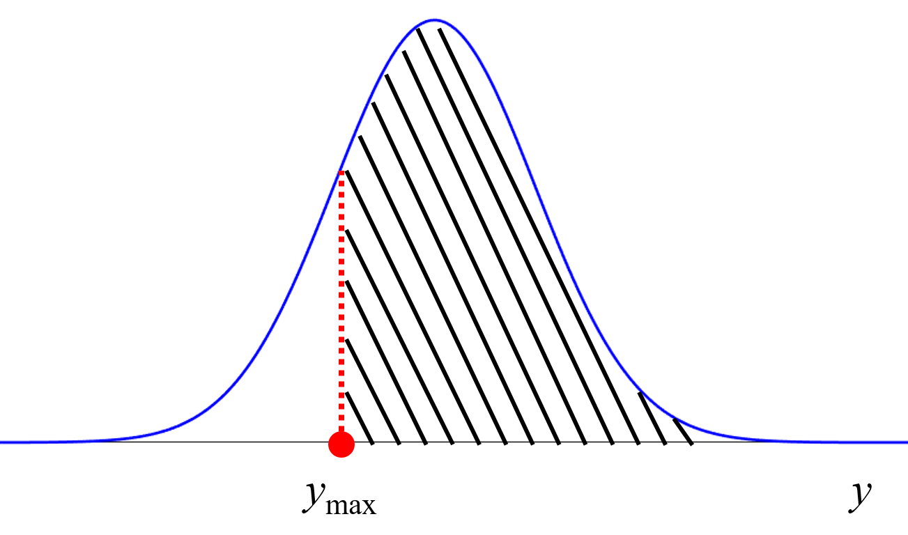

Select the candidate of X with the highest acquisition function using the Gaussian process regression model with BO
Parameters :
- X : numpy.array or pandas.DataFrame, shape (n_samples, n_features)
(オートスケーリング後の) X のトレーニングデータ - y : numpy.array or pandas.DataFrame, shape (n_samples,)
(オートスケーリング後の) Y のトレーニングデータ - candidates_of_X: numpy.array or pandas.DataFrame (n_test_samples, n_features)
(オートスケーリング後の) Y が不明な X のデータ - acquisition_function_flag: int
1: Mutual information (MI), 2: Expected improvement(EI),
3: Probability of improvement (PI) [0: y の推定値] - cumulative_variance: numpy.array or pandas.DataFrame, default None
MI のための (更新される) サンプルごとの分散の値
Returns :
- selected_candidate_number : int
選ばれた candidates_of_X の 1 サンプルの番号 - selected number of candidates_of_X
選ばれた candidates_of_X の 1 サンプル - cumulative_variance: numpy.array
MI のための (更新される) サンプルごとの分散の値
Examples :
- demo_bayesian_optimization.py
- demo_bayesian_optimization_multiple_y.py (目的変数が複数、実際は上の関数を使用していません。このプログラムの使い方に関しては こちら をご覧ください)
class dcekit.learning.SemiSupervisedLearningLowDimension(base_estimator=None, base_dimension_reductioner=None, x_unsupervised=None,
autoscaling_flag=True, cv_flag=False, ad_flag=False, k=5, within_ad_rate=0.997)
scikit-learn に準拠しています (GridSearchCV や cross_val_predict を使えます)
次元削減による半教師あり学習 (Semi-Supervised Learning) + AD による教師なしサンプルの選択
Parameters :
- base_estimator: object of model in scikit-learn or object of GridSearchCV
sklearn で fit する前のモデルもしくは、クロスバリデーションするときの GridSearchCV。GridSearchCV のときには cv_flag を True にしてください - base_dimension_reductioner: object of model in scikit-learn
sklearn で fit する前の低次元化のモデル。PCA のように ‘transform’ があるものにしてください。DCEKit の GTM も使えます - x_unsupervised : numpy.array or pandas.DataFrame, shape (n_samples, n_features)
x の教師なしデータ - autoscaling_flag : boolean, default True
True のときオートスケーリングして、False のときしません - cv_flag: boolen, default False
True のとき base_estimator を GridSearchCV のオブジェクトにしてください - ad_flag: boolen, default False
True のとき、教師ありデータを用いて k 最近傍法 (k-NN) で AD を設定し、AD 内のサンプルのみ教師なしデータとして使用します
ScienceDirectwww.sciencedirect.com - k: int, default 5
k-NN における k の値。ad_flag が True のときのみ使用します - within_ad_rate: float, default 0.997
AD 内となる教師ありデータの割合。ad_flag が True のときのみ、AD のしきい値を設定するために使用します

Attributes :
- combined_x: numpy.array, shape (n_samples, n_features)
教師ありデータと (AD で選択された) 教師なしデータを縦に繋げたデータ - transformed_x: numpy.array, shape (n_samples, n_latent_variables)
低次元化された、教師ありデータと (AD で選択された) 教師なしデータが縦に繋がったデータ
Methods:
- fit(self, x, y) : Fit model
- predict(self, x) : Predict y-values of samples
fit(self, x, y) : Fit model
Parameters :
- x: numpy.array, shape (n_samples, n_features)
モデル構築のための x のデータ - y : numpy.array, shape (n_samples,)
モデル構築のための y のデータ
Returns :
- self : returns an instance of self
scikit-learn と同じです
predict(self, x) : Predict y-values of samples
Parameters :
- x: numpy.array, shape (n_samples, n_features)
モデルで予測するための x のデータ
Returns :
- estimated_y : numpy.array, shape (n_samples,)
y の予測値
Examples :
- demo_semi_supervised_learning_low_dim_no_hyperparameters.py (GP, OLS のようにハイパーパラメータのないモデリング手法)
- demo_semi_supervised_learning_low_dim_no_hyperparameters_with_ad.py (GP, OLS のようにハイパーパラメータのないモデリング手法、AD を考慮して教師なしデータを選択)
- demo_semi_supervised_learning_low_dim_with_hyperparameters.py (PLS, SVR のようにハイパーパラメータがあるモデリング手法)
- demo_semi_supervised_learning_low_dim_with_hyperparameters_with_ad.py (PLS, SVR のようにハイパーパラメータがあるモデリング手法、AD を考慮して教師なしデータを選択)
class dcekit.learning.TransferLearningSample(base_estimator=None, x_source=None, y_source=None, autoscaling_flag=False, cv_flag=False)
scikit-learn に準拠しています (GridSearchCV や cross_val_predict を使えます)
サンプルを転移するタイプの転移学習 (Transfer Learning)

Parameters :
- base_estimator: object of model in scikit-learn or object of GridSearchCV
sklearn で fit する前のモデルもしくは、クロスバリデーションするときの GridSearchCV。GridSearchCV のときには cv_flag を True にしてください - x_source: numpy.array or pandas.DataFrame, shape (n_samples, n_features)
転移させる (サンプル数の多い) x のデータ - y_source: numpy.array or pandas.DataFrame, shape (n_samples,)
転移させる (サンプル数の多い) y のデータ - autoscaling_flag : boolean, default False
True のときオートスケーリングして、False のときしません - cv_flag: boolen, default False
True のとき base_estimator を GridSearchCV のオブジェクトにしてください
Attributes :
- combined_x: numpy.array, shape (n_samples, n_features)
転移させるデータとターゲットのデータを、0 で繋げた x のデータ - combined_y: numpy.array, shape (n_samples,)
転移させるデータとターゲットのデータを、繋げた y のデータ
Methods:
- fit(self, x, y) : Fit model
- predict(self, x, target_flag=True) : Predict y-values of samples
fit(self, x, y) : Fit model
Parameters :
- x: numpy.array, shape (n_samples, n_features)
モデル構築のための x のデータ - y : numpy.array, shape (n_samples,)
モデル構築のための y のデータ
Returns :
- self : returns an instance of self
scikit-learn と同じです
predict(self, x, target_flag=True) : Predict y-values of samples
Parameters :
- x: numpy.array, shape (n_samples, n_features)
モデルで予測するための x のデータ - target_flag : boolean, default True
True のときターゲットのデータの y を値を予測し、False のときサポート用の (転移させる、サンプル数の多い) データの y の値を予測
Returns :
- estimated_y : numpy.array, shape (n_samples,)
y の予測値
Examples :
- demo_transfer_learning_no_hyperparameters.py (GP, OLS のようにハイパーパラメータのないモデリング手法)
- demo_transfer_learning_with_hyperparameters.py (PLS, SVR のようにハイパーパラメータがあるモデリング手法)
class dcekit.learning.DCEBaggingRegressor(base_estimator=None, n_estimators=100, max_features=1.0, autoscaling_flag=False,
cv_flag=False, robust_flag=True, random_state=None)
scikit-learn に準拠しています (GridSearchCV や cross_val_predict を使えます)
バギングと回帰分析でのアンサンブル学習 (Ensemble Learning based on Bagging and Regression)
Parameters :
- base_estimator: object of model in scikit-learn or object of GridSearchCV
sklearn で fit する前のモデルもしくは、クロスバリデーションするときの GridSearchCV。GridSearchCV のときには cv_flag を True にしてください - n_estimators: int, default 100
サブデータセットやサブモデルの数 - max_features: int or float, default 1.0
整数のときはサブデータセットを使用する際に選択する説明変数の数、少数のときはサブデータセットを使用する際に選択する説明変数の数の割合 - autoscaling_flag : boolean, default True
True のときはサブデータセットごとにオートスケーリングして、False のときしません - cv_flag: boolean, default False
True のとき base_estimator を GridSearchCV のオブジェクトにしてください - robust_flag: boolean, default True
True のときは中央値や中央絶対偏差を使用し、False のときは平均値や標準偏差を使用します - random_state : int, default None
再現性のため乱数のシードを固定します
Attributes :
- estimators_: list, shape(n_estimators,)
サブモデルのオブジェクト - estimators_features_: list, shape (n_estimators,)
サブデータセットごとの選択された説明変数の番号 - x_means_: list, shape (n_estimators,)
サブデータセットごとの x の平均値 - x_stds_: list, shape (n_estimators,)
サブデータセットごとの x の標準偏差 - y_means_: list, shape (n_estimators,)
サブデータセットごとの y の平均値 - y_stds_: list, shape (n_estimators,)
サブデータセットごとの y の標準偏差
Methods:
- fit(self, x, y) : Fit model
- predict(self, x, return_std=False) : Predict y-values of samples
fit(self, x, y) : Fit model
Parameters :
- x: numpy.array, shape (n_samples, n_features)
モデル構築のための x のデータ - y : numpy.array, shape (n_samples,)
モデル構築のための y のデータ
Returns :
- self : returns an instance of self
scikit-learn と同じです
predict(self, x, return_std=False) : Predict y-values of samples
Parameters :
- x: numpy.array, shape (n_samples, n_features)
モデルで予測するための x のデータ - return_std: boolean, default False
True のとき予測値の中央絶対偏差もしくは標準偏差も一緒に出力
Returns :
- estimated_y : numpy.array, shape (n_samples,)
y の予測値 - estimated_y_std : numpy.array, shape (n_samples, n_estimators)
y の予測値の中央絶対偏差もしくは標準偏差
Examples :
- demo_bagging_regression_no_hyperparameters (GP, OLS のようにハイパーパラメータのない回帰分析手法)
- demo_bagging_regression_with_hyperparameters.py (PLS, SVR のようにハイパーパラメータがある回帰分析手法)
class dcekit.learning.DCEBaggingClassifier(base_estimator=None, n_estimators=100, max_features=1.0, autoscaling_flag=False,
cv_flag=False, random_state=None)
scikit-learn に準拠しています (GridSearchCV や cross_val_predict を使えます)
バギングとクラス分類でのアンサンブル学習 (Ensemble Learning based on Bagging and Classification)
Parameters :
- base_estimator: object of model in scikit-learn or object of GridSearchCV
sklearn で fit する前のモデルもしくは、クロスバリデーションするときの GridSearchCV。GridSearchCV のときには cv_flag を True にしてください - n_estimators: int, default 100
サブデータセットやサブモデルの数 - max_features: int or float, default 1.0
整数のときはサブデータセットを使用する際に選択する説明変数の数、少数のときはサブデータセットを使用する際に選択する説明変数の数の割合 - autoscaling_flag : boolean, default True
True のときはサブデータセットごとにオートスケーリングして、False のときしません - cv_flag: boolean, default False
True のとき base_estimator を GridSearchCV のオブジェクトにしてください - random_state : int, default None
再現性のため乱数のシードを固定します
Attributes :
- estimators_: list, shape(n_estimators,)
サブモデルのオブジェクト - estimators_features_: list, shape (n_estimators,)
サブデータセットごとの選択された説明変数の番号 - x_means_: list, shape (n_estimators,)
サブデータセットごとの x の平均値 - x_stds_: list, shape (n_estimators,)
サブデータセットごとの x の標準偏差 - class_types_: list, shape (n_classes,)
クラスの種類
Methods:
- fit(self, x, y) : Fit model
- predict(self, x, return_probability=False) : Predict y-values of samples
fit(self, x, y) : Fit model
Parameters :
- x: numpy.array, shape (n_samples, n_features)
モデル構築のための x のデータ - y : numpy.array, shape (n_samples,)
モデル構築のための y のデータ
Returns :
- self : returns an instance of self
scikit-learn と同じです
predict(self, x, return_probability=False) : Predict y-values of samples
Parameters :
- x: numpy.array, shape (n_samples, n_features)
モデルで予測するための x のデータ - return_probability: boolean, default False
True のとき各クラスの確率 (そのクラスと推定したサブモデルの数の割合) も一緒に出力
Returns :
- estimated_y : numpy.array, shape (n_samples,)
y の予測値 - estimated_y_probability : pd.DataFrame, shape (n_samples, n_classes)
各クラスの確率 (そのクラスと推定したサブモデルの数の割合)
Examples :
- demo_bagging_classification_no_hyperparameters (LDA のようにハイパーパラメータのないクラス分類手法)
- demo_bagging_classification_with_hyperparameters.py (SVM のようにハイパーパラメータがあるクラス分類手法)
dcekit.learning.ensemble_outlier_sample_detection(base_estimator, x, y, cv_flag, n_estimators=100, iteration=30,
autoscaling_flag=True, random_state=None)
アンサンブル学習に基づく外れサンプル検出 (Ensemble Learning Outlier sample detection, ELO)
Parameters :
- base_estimator: object of model in scikit-learn or object of GridSearchCV
sklearn で fit する前のモデルもしくは、クロスバリデーションするときの GridSearchCV。GridSearchCV のときには cv_flag を True にしてください - x: numpy.array, shape (n_samples, n_features)
(外れサンプルが含まれる可能性のある) モデル構築のための x のデータ - y : numpy.array, shape (n_samples,)
(外れサンプルが含まれる可能性のある) モデル構築のための y のデータ - cv_flag: boolean, default False
True のとき base_estimator を GridSearchCV のオブジェクトにしてください - n_estimators: int, default 100
サブデータセットやサブモデルの数 - iteration: int, default 30
最大の繰り返し回数 - autoscaling_flag : boolean, default True
True のときはサブデータセットごとにオートスケーリングして、False のときしません - random_state : int, default None
再現性のため乱数のシードを固定します
Returns :
- outlier_sample_flags : numpy.array, shape (n_samples,)
外れサンプルの番号だけ TRUE になっているベクトル
Examples :
- demo_elo_pls.py (PLS のアンサンブル)
class dcekit.validation.ApplicabilityDomain(method_name=’ocsvm’, rate_of_outliers=0.01, gamma=’auto’, nu=0.5, n_neighbors=10,
metric=’minkowski’, p=2)
モデルの適用範囲・適用領域 (Applicability Domain, AD) [データ密度]
Parameters :
- method_name: str, default ‘ocsvm’
AD を設定する手法の名前。
‘knn’: k最近傍法(k-NN),
‘lof’: Local Outlier Factor (LOF)
‘ocsvm’: One-Class Support Vector Machine (OCSVM) - rate_of_outliers: float, default 0.01
外れサンプルの割合。AD の指標は、0 より小さいときに AD 外となりますが、しきい値としての 0 を決めるために使われます - gamma : (only for ‘ocsvm’) float, default ’auto’
OCSVM におけるガウシアンカーネルの γ。’auto’ にするとグラム行列の分散を最大化するように自動的に最適化されます。
OneClassSVMGallery examples: Outlier detection on a real data set Species distribution modeling One-Class SVM versus One-Class SVM ...scikit-learn - nu : (only for ‘ocsvm’) float, default ’0.5’
OCSVM における ν。 - n_neighbors: (only for ‘knn’ and ‘lof’) int, default 10
k-NN や LOF における考慮する近傍サンプルの数
NearestNeighborsGallery examples: Approximate nearest neighbors in TSNEscikit-learn - metric : string or callable, default ‘minkowski’
距離の指標。詳しくはこちら
NearestNeighborsGallery examples: Approximate nearest neighbors in TSNEscikit-learn - p : integer, default 2
Minkowski 距離の p。p=2 でユークリッド距離。詳しくはこちら
NearestNeighborsGallery examples: Approximate nearest neighbors in TSNEscikit-learn


Methods:
- fit(self, x) : Set AD
- predict(self, x) : Predict AD-values
fit(self, x) : Set AD
Parameters :
- x: numpy.array, shape (n_samples, n_features)
AD を設定するための x のデータ
Returns :
- self : returns an instance of self
scikit-learn と同じです
predict(self, x) : Predict AD-values
Parameters :
- x: numpy.array, shape (n_samples, n_features)
AD の指標の値を予測するための x のデータ
Returns :
- ad_values : numpy.array, shape (n_samples,)
0 より小さいと AD の外を意味するように調整された、AD の指標の値。OCSVM や LOF ではそれぞれの出力の値であり、k-NNでは平均距離の逆数です
Examples :
- demo_ad.py (回帰分析手法は GP)
class dcekit.validation.DCEGridSearchCV(estimator, param_grid, *, scoring=None, n_jobs=None, refit=True, cv=None, verbose=0, pre_dispatch=”2*n_jobs”, error_score=np.nan, return_train_score=False, random_state = None, shuffle = True, display_flag = False)
グリッドサーチとクロスバリデーションによるハイパーパラメータ最適化
Parameters :
基本的に GridSearchCV, KFold, and StratifiedKFold におけるパラメータと同じです。
- GridSearchCV : https://scikit-learn.org/stable/modules/generated/sklearn.model_selection.GridSearchCV.html
- KFold : https://scikit-learn.org/stable/modules/generated/sklearn.model_selection.KFold.html
- StratifiedKFold : https://scikit-learn.org/stable/modules/generated/sklearn.model_selection.StratifiedKFold.html#sklearn.model_selection.StratifiedKFold
Methods:
- fit(self, x, y) : Hyperparameter optimization with grid search and cross-validation
- predict(self, x) : Predict y with the model with the optimized hyperparameters
fit(self, x, y) : Hyperparameter optimization with grid search and cross-validation
Parameters : GridSearchCV と同じです。
Returns : GridSearchCV と同じです。
predict(self, x) : Predict y with the model with the optimized hyperparameters
Parameters : GridSearchCV と同じです。
Returns : GridSearchCV と同じです。
Examples :
- demo_DCEGridSearchCV_classification.py (クラス分類、SVM)
- demo_DCEGridSearchCV_regression.py (回帰分析、Elastic Net)
今後も DCEKit を拡張しだい、こちらも更新いたします。
以上です。
質問やコメントなどありましたら、twitter, facebook, メールなどでご連絡いただけるとうれしいです。